Speaker
Description
In magnetically confined fusion devices, nonlinear wave-wave interaction has been noticed to play important roles in the production of new modes. On NSTX, nonlinear interactions among low-frequency energetic particle modes (EPMs) and high-frequency toroidal Alfvén modes (TAEs) have been reported $[1]$. On JET, a 3/2 neoclassical tearing mode (NTM) is stabilized through the nonlinear coupling among 3/2, 4/3 and 7/5 modes $[2]$. On HL-2A, high frequency coherent modes can be driven by nonlinear wave-wave coupling $[3]$. Routinely, bispectral analysis is applied to detect the nonlinear interaction $[4]$. However, a number of statistical ensembles are necessary for the bispectral analysis. Here, we propose to use Hilbert transform $[5]$ for the analysis of nonlinear wave-wave interaction without many ensembles.
Two spontaneously excited waves could generate new waves through nonlinear interaction. Supposing there are two waves b and c, wave b is cos$\it{\theta}_b$ = cos(2$\pi\it{f}_bt+\it{\phi}_b$), and wave c is cos$\it{\theta}_c$ = cos(2$\pi\it{f}_ct+\it{\phi}_c$). Here, $\it{\theta}_b$ and $\it{\theta}_c$ are the time dependent instantaneous phases, and $\it{\phi}_b$ and $\it{\phi}_c$ are the initial phases. If nonlinear interaction exists between b and c, the generated new wave d should be the product of the two waves, cos $\it{\theta}_d$ = cos $\it{\theta}_b$ cos$\it{\theta}_c$ = cos(2$\pi(\it{f}_b+\it{f}_c$))t+$\it{\phi}_b$+$\it{\phi}_c$)) + cos(2$\pi(\it{f}_b-\it{f}_c$)t+$\it{\phi}_b$-$\it{\phi}_c$))/2. Wave d will have the frequency components of $\it{f}_b+\it{f}_c$, and the initial phases have to obey $\it{\phi}_d$ = $\it{\phi}_b$+$\it{\phi}_c$. This condition is actually $\it{\theta}_d$ = $\it{\theta}_b$+$\it{\theta}_c$. For simplification, we focus on the case of $\it{f}_d$ = $\it{f}_b+\it{f}_c$, the analysis of $\it{f}_d$ = $\it{f}_b-\it{f}_c$ is actually in a similar way. Let’s generate a synthetic signal of 10 ms with a sampling rate of 1 MHz, including three waves b, c, d and some random noise. The frequencies of the three waves are $\it{f}_b$ = 30 kHz, $\it{f}_c$ = 95 kHz and $\it{f}_d$ = $\it{f}_b+\it{f}_c$ = 125 kHz. If wave d is the result of mode coupling between wave b and wave c, the phase relation $\it{\theta}_d$ = $\it{\theta}_b$+$\it{\theta}_c$, i.e. $\it{\theta}_d-\it{\theta}_c$ = $\it{\theta}_b$ has to be satisfied. In Fig. 1(a), wave b (blue curve), wave c (red curve), wave d (orange curve) and the sum of b, c, d and a random noise (purple curve) are plotted. In Fig. 1(b), the power spectral density (PSD) of the purple signal in Fig. 1(a) shows the peaks of three waves at 30 kHz, 95 kHz, and 125 kHz. Supposing $\it{\theta}_b$ jumps at 0.5 ms, 1 ms, (in the intervals of 0.5 ms) to 9.5 ms (while $\it{\theta}_c$ does not jump), to satisfy the phase relation $\it{\theta}_d-\it{\theta}_c$ = $\it{\theta}_b$, $\it{\theta}_d$ has to jump at the same timings. In Fig. 1(a), the phase jumps of wave b and wave d at 0.5ms are labeled. The phase difference between wave d and wave c $\Delta\it{\theta}_{dc}$ = $\it{\theta}_d-\it{\theta}_c$, and the phase of wave b $\it{\theta}_b$ for Fig. 1(c) are shown in Fig. 1(d). The jump of both $\it{\theta}_{dc}$ and $\it{\theta}_b$ at 0.5ms is clearly observed. Due to the phase relation, the two phases are locked together. The fast fourier t ransform (FFT) bicoherence spectrogram is shown in Fig. 1(d). A bright spot is observed at ($\it{\theta}_c$, $\it{\theta}_b$) = (95, 30) kHz, indicating that the nonlinear coupling exists among waves b, c and d.
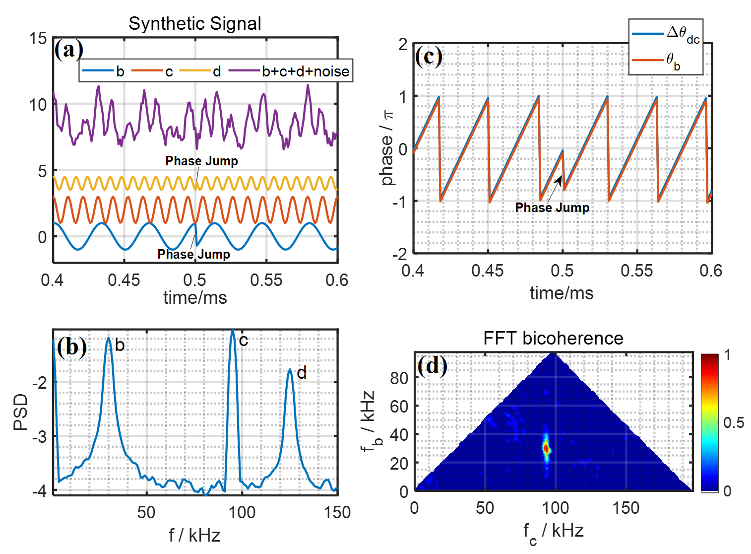
Fig. 2 (a) and (b) are the power spectrogram and the bicoherence spectrogram of the mirnov coil signal, respectively. The nonlinear coupling among AM1, AM2 and TM has been identified by observing the bright spot at (f1, f2) = (129 kHz, 10 kHz) and (f1, f2) = (139 kHz, 10 kHz). $\it{\theta}_{AM1}$, $\it{\theta}_{AM2}$ and $\it{\theta}_{TM}$ stand for the instantaneous phases of AM1, AM2 and TM, respectively. In Fig. 2 (b), the blue curve is the phase delay between AM1 and AM2, i.e. $\Delta\it{\theta}_{12}$ = $\it{\theta}_{AM1}-\it{\theta}_{AM2}$, and the red curve is $\it{\theta}_{TM}$. We could observe that $\Delta\it{\theta}_{12}$ and $\Delta\it{\theta}_{TM}$ are roughly synchronized with each other, and the maximum value of cross-correlation coefficient between them r($\Delta\it{\theta}_{12}$, $\it{\theta}_{TM}$) reaches 0.84, as shown in Fig. 2 (c). As a counter-example, we check the phases of AM1, AM2 during 696-698 ms and 8-12 kHz band-passed waveform during 676-678 ms. The first two waves and the last wave are in different timings, and the TM during 676-678 ms is not in 8-12 kHz, as shown in the power spectrogram in Fig. 2 (b). Therefore there are basically no nonlinear coupling among these three modes. The phase difference between AM1 and AM2 during 696-698ms $\Delta\it{\theta}_{12}$, and 8-12 kHz band-passed wave during 676-678ms $\it{\theta}_{8-12kHz}$ have been checked in Fig. 2 (e). In this figure, the phases are not synchronized at all, which means that nonlinear interaction does not exist. The maximum value of cross-correlation coefficient between $\Delta\it{\theta}_{12}$ and $\it{\theta}_{8-12kHz}$, r($\Delta\it{\theta}_{12}$, $\it{\theta}_{8-12kHz}$) is only 0.1, as shown in Fig. 2 (f).
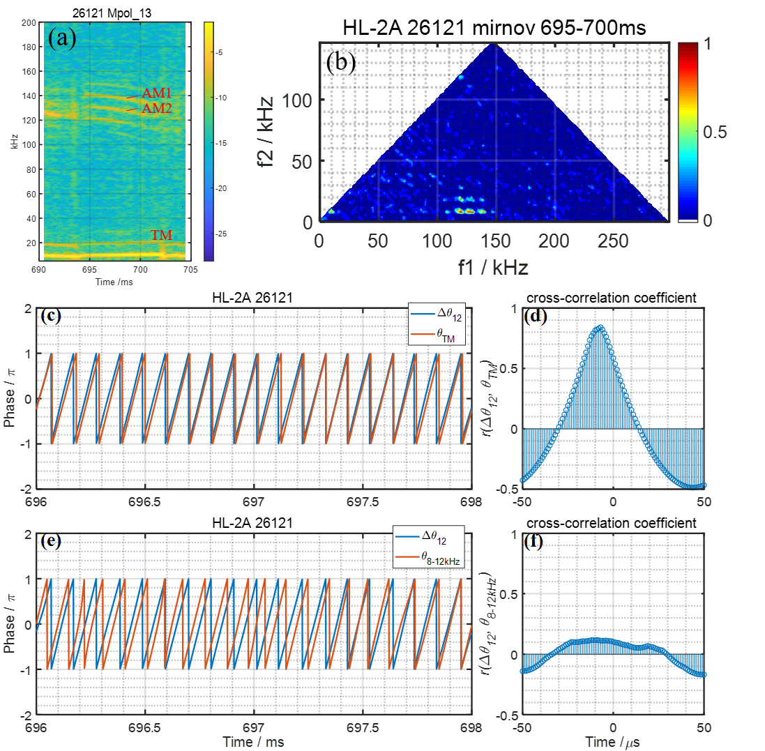
Figure 2: (a) The power spectrogram; (b) The FFT bicoherence spectrogram; (c) The blue curve is the time evolution of $\Delta\it{\theta}_{12}$, and the red curve is the time evolution of $\it{\theta}_{TM}$. (d) The time evolution of r($\Delta\it{\theta}_{12}$, $\it{\theta}_{TM}$) during [-50, 50]$\mu$s. (e) The blue curve and the red curve are the time evolutions of $\Delta\it{\theta}_{12}$, and $\it{\theta}_{8-12kHz}$, respectively. (f) The time evolution of r($\Delta\it{\theta}_{12}$, $\it{\theta}_{TM}$) during [-50, 50]$\mu$s.
As a summary, the Hilbert transform allows us to track the phase of a mode without many ensembles. In our work, the nonlinear interactions among the 139kHz and 129kHz AMs and the 10kHz TM on HL-2A were checked using phase tracking with Hilbert Transform. Results show that the phase delay between two AMs $\Delta\it{\theta}_{12}$ is approximately synchronized with the phase of TM $\it{\theta}_{TM}$ and the maximum of the normalized cross-correlation is 0.84. In a counter example, the maximum of normalized cross-correlation is only 0.18.
This work was supported by National Key R&D Program of China under Grant Nos. 2018YFE0310200 and 2017YFE0301203, National Natural Science Foundation of China under Grant No. 11775069, Sichuan Science and Technology Program Grant Nos. 19GJHZ0154.
References:
$[1]$ Crocker N A, Peebles W A, Kubota S, Fredrickson E D, Kaye S M, LeBlanc B P and Menard J E 2006 Phys. Rev. Lett. 97 045002
$[2]$ Raju D, Sauter O and Lister J B 2003 Plasma Phys. Control. Fusion 45 369
$[3]$ Shi P W et al 2019 Nucl. Fusion 59 086001
$[4]$ Kim Y C and Powers E J 1979 IEEE Trans. Plasma Sci. 7 120
$[5]$ Ohshima S et al 2014 Rev. Sci. Instrum. 85 11E814
| Affiliation | Southwestern Institute of Physics |
|---|---|
| Country or International Organization | China |
